Systems with few degrees of freedom#
Examples with 1 degree of freedom#
Non-linear rigid pendulum#
We consider the very simple mechanical system of a mass hung to a rigid bar free to oscillate in one dimension. Let’s start by an exercise.
Exercise 1
Prove that the dynamics of this system can be describe by this equation:
where \(\Omega_g = \sqrt{g/R}\) and \(f_d\) is a dissipation frequency.
Definition fixed points
Fixed points are points (values of the variables) for with \(\dot\theta = 0\).
Exercise 2
What are the fixed points of this equations?
Answer: The two fixed points are \(\theta_0 = 0\) and \(\theta_1 = \pi\).
To study the stability of a fixed point, we have to linearize the equation around this fixed point. We write the variable as the sum of a fixed points value plus a small perturbation: \(\theta = \theta_f + {\varepsilon}\) and we neglect the nonlinear terms involving \({\varepsilon}^2\). We then can look for a solution of the obtained linear equation in the form \({\varepsilon}\propto e^{\sigma t}\). We then obtain an equation for the growth rate of the perturbation \(\sigma\).
First fixed point, \(\theta_0 = 0\)#
\(\sigma_\pm = -f_d \pm \sqrt{f_d^2 - \Omega_g^2}\)
Case \(f_d \ll \Omega_d\): \(\sigma_{\pm r} \simeq - f_d < 0\) and \(\sigma_{\pm i} = \pm \Omega_g\).
Stable…
Second fixed point, \(\theta_1 = \pi\)#
One unstable mode…
Non-linear rotating pendulum#
Let’s consider the same mechanical system but with a global system rotation. A picture of an experiment of such rotating pendulum is shown in Fig. 5.
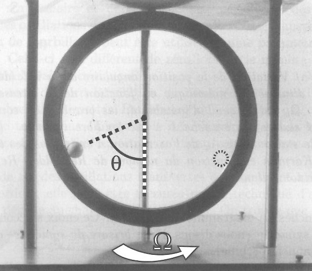
Fig. 5 Picture of an experiment of a rotating pendulum.#
Try to show that the equation describing the dynamics of the rotating pendulum can be written as
We now have three fixed points: \(\theta_0 = 0\), \(\theta_1 = \pi\) and \(\theta_\pm = \pm \arccos(\Omega_g^2 / \Omega^2)\) (only if \(\Omega > \Omega_g\)).
Stability of the first fixed point \(\theta_0 = 0\)#
\(\theta = \theta_0 + \theta'\).
\(\sigma_0^2 = \Omega^2 - \Omega_g^2\).
Stability of the other fixed point#
\(\cos \theta_\pm = (\Omega_g / \Omega)^2\)
We can write the governing equation as:
We write the angle as \(\theta = \theta_\pm + \theta'\) and we develop \(\cos\theta\) and \(\sin\theta\) around \(\theta_\pm\):
By using the trigonometry equality \(\sin^2\theta_\pm = 1 - \cos^2\theta_\pm\), we find
Therefore, these fixed points are unstable when \(\Omega < \Omega_g\) and stable (oscillations) when \(\Omega > \Omega_g\).
Close to the transition \(\tilde \Omega \ll 1\)#
Non dimensional control parameter:
\(\Omega / \Omega_g = 1 + \tilde \Omega\).
In the limit \(\tilde \Omega \ll 1\), we have \(\cos\theta_\pm = (\Omega / \Omega_g)^{-2} \Rightarrow 1 - \theta^2 / 2 = 1 - 2 \tilde \Omega \Rightarrow \theta_\pm \simeq \pm 2 \sqrt{\tilde \Omega}\).
We can plot the transition diagram close to the bifurcation. This is a Pitchfork bifurcation.
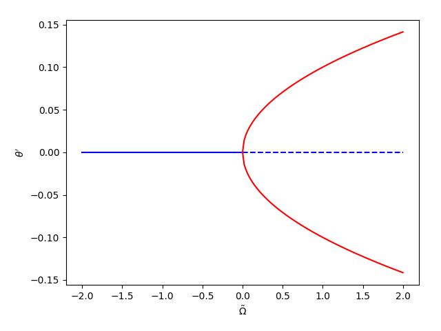
Fig. 6 Supercritical pitchfork bifurcation: solid lines represent stable points and the dashed line represents an unstable one.#
Introduction of the concepts of supercritical and subcritical instabilities#
Fig. 7 shows two diagrams corresponding to supercritical and subcritical bifurcations, respectively. The first bifurcation of the wake of a cylinder is supercritical (similar to the rotating pendulum). The transition to turbulence in a straight tube is due to a subcritical instability (hysteresis).
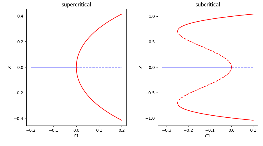
Fig. 7 Bifurcation diagrams for a supercritical instability (left) and a subcritical instability (right).#
Example with 2 degrees of freedom (linearization, diagonalization, eigenmodes)#
We consider the predator–prey model, also known as the Lotka–Volterra equations:
where \(X(t)\) and \(Y(t)\) are two functions of time representing species of preys and predators, respectively. The parameters \(A\), \(B\), \(C\) and \(D\) are real and positive. This model is very simple, which will help us to introduce the concepts of fixed points, linearization, diagonalization of a linear system, eigenvalues and eigenmodes.
Fixed points#
A first simple step when studying a dynamical system consists in finding fixed points, i.e. points for which the system is stationary (\((\dot X,\ \dot Y) = (0,\ 0)\)). To find the fixed points, let’s factorize the system of equation:
The first trivial fixed point is \((X,\ Y) = (0,\ 0)\) and corresponds to the extinction of the two species. We see that there is also a non-trivial fixed point: \((X,\ Y) = (C/D,\ A/B)\).
Stability of the fixed points#
A second step is to study the stability of the two fixed points. We first have to linearise the equations around a fixed point. We consider an infinitesimal perturbation so we write the solution in the form \(X = X_f + x\) and \(Y = Y_f + y\).
For the first fixed point, it is trivial. The linearized equations are
and can be written as \(\dot V = J V\), with
\(J\) is the Jacobian matrix of the system. We need to find eigenvalues and eigenmodes of this matrix, i.e. vector \(V_i\) such that \(\sigma_i V_i = J V_i\). Since, \(J\) is in this case already diagonal, it is trivial. The eigenvalues are \(\sigma_1 = A\) and \(\sigma_2 = -C\) and the eigenvectors are
Since \(A\) and \(C\) are both positive, this fixed point is unstable and it is a saddle point (\(\sigma_1 > 0\) and \(\sigma_2 < 0\)).
We now consider an infinitesimal perturbation around the second fixed point \((X,\ Y) = (C/D,\ A/B)\). The linearized equations can be written as \(\dot V = J V\) with the Jacobian matrix
This time, it is not diagonal so we have to work a little bit more. The solvability condition is
with \({\boldsymbol{1}}\) the identity matrix, which gives us \(\sigma_\pm = \pm i \sqrt{AC}\), which means that the fixed point is elliptic (characterizes the shape of the orbits close to the fixed point). By injecting the value of the eigenvalue in the linearized equations, we find the eigenvectors:
Phase space: place the two fixed points in the space \((X,\ Y)\). Plot (approximately) some trajectories.
Conserved quantity: Check that the quantity
is conserved along the trajectories.
Periodic orbits and predictability: The orbits are periodic. The state of the system remains predictable for all times. There is no sensitivity to initial conditions.
Example with 3 degrees of freedom : the Lorenz model (chaos)#
We have just studied a deterministic system with 2 degrees of freedom. We have seen that the system is predictable.
We are going to see that something very different happens for a very similar deterministic system with just 1 more degree of freedom, the Lorenz model inspired by the convection in the atmosphere:
Find the fixed points…
There is no periodic orbit and there is a strong sensitivity to initial conditions, which is called the “butterfly” effect. This is an example of chaos for systems characterized by a small number of degrees of freedom. We see that we do not need many degrees of freedom to get unpredictable system.
Revision on simple instabilities#
We consider the dynamical equation
where \(C_1\), \(C_2\) and \(C_3\) are three parameters.
Case \(C_3 = C_5 = -1\)#
(a) Write down the equation for the growth rate \(\dot X / X\) for this case. (b) Draw schematic representations of the growth rate as a function of \(X\) for two values of the control parameter \(C_1\). One value for which \(\dot X / X\) is always negative and another value for which \(\dot X / X\) is positive close to \(X = 0\).
(c)If \(X<0\) and \(\dot X / X > 0\), \(|X|\) increases or decreases? (d) Show the positions of stable fixed points with circles and the position of unstable fixed points with crosses.Draw a schematic representation of the bifurcation diagram as a function of the control parameter \(C_1\). Draw the stable branches as continuous lines and the unstable branches as dashed lines.
Which type of bifurcation is it? Cite a physical example for which such type of instability is important.