Introduction

Example of turbulent signals

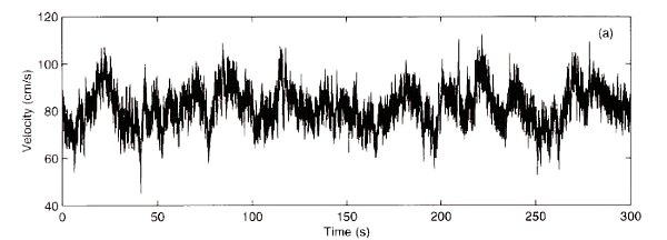
Fig. 19 Typical turbulent velocity signal \(u(t)\) obtained for example with a hot wire for a very large Reynolds number.

• Unpredictable (chaos at high number of degrees of freedom).

• Multi-scale (time and space). Wideband spectra.

• Large Reynolds number. Strongly nonlinear.

Turbulence study is a lot about analysis and understanding the characteristics of such flow signal \({\boldsymbol{u}}({\boldsymbol{x}}, t)\). What can we do with such signals?

• Average and filtering \({\langle u \rangle}\).

• Energy \({\langle {\boldsymbol{u}}^2/2 \rangle}\).

• Time and space correlations. Structure functions.

• Spectra.

A simple model: Richardson cascade, dissipation rate

\(\varepsilon\)

At very large Reynolds number, the drag coefficient is constant… This tends to indicate that the rate of dissipation of the energy is not a function of the viscosity! The equation for the local kinetic energy per mass unit is:

\[{\text{D}_t}{\boldsymbol{u}}^2/2 = - {\boldsymbol{u}}\cdot{\boldsymbol{\nabla}}p + \nu {\boldsymbol{u}}\cdot {\boldsymbol{\nabla}}^2 {\boldsymbol{u}}.\]

The dissipation term is \({\varepsilon}({\boldsymbol{x}}, t) = \nu {\boldsymbol{u}}\cdot {\boldsymbol{\nabla}}^2 {\boldsymbol{u}}\). It is proportional to the viscosity so it should tends towards 0 when \(\nu\) tends towards 0, but it is actually constant when \(\nu\) tends towards 0! This surprising limit can be explained only by the fact that the size of the smallest structures in the flow decreases when \(\nu\) tends towards 0 such that the rate of dissipation of the energy is constant.

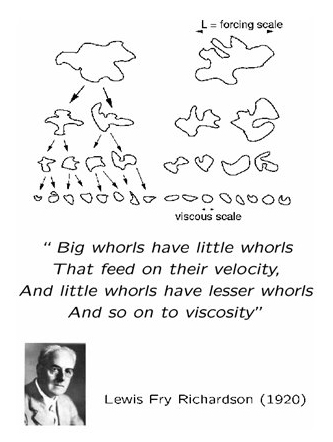
Fig. 20 A simple model of turbulence introduced by physicist Lewis Richardson in 1920. Credit: Antonio Celani.